My Research Ambition
I’m aiming to achieve the optimal trade-off between theory and learning.
Design algorithms that benefit both from rigorness of theory and flexibility of ML for different applications from combinatorial optimization to derivative pricing.
For a more detailed write-up of this research philosophy, see my blog post: Theory-Embedding Learning.
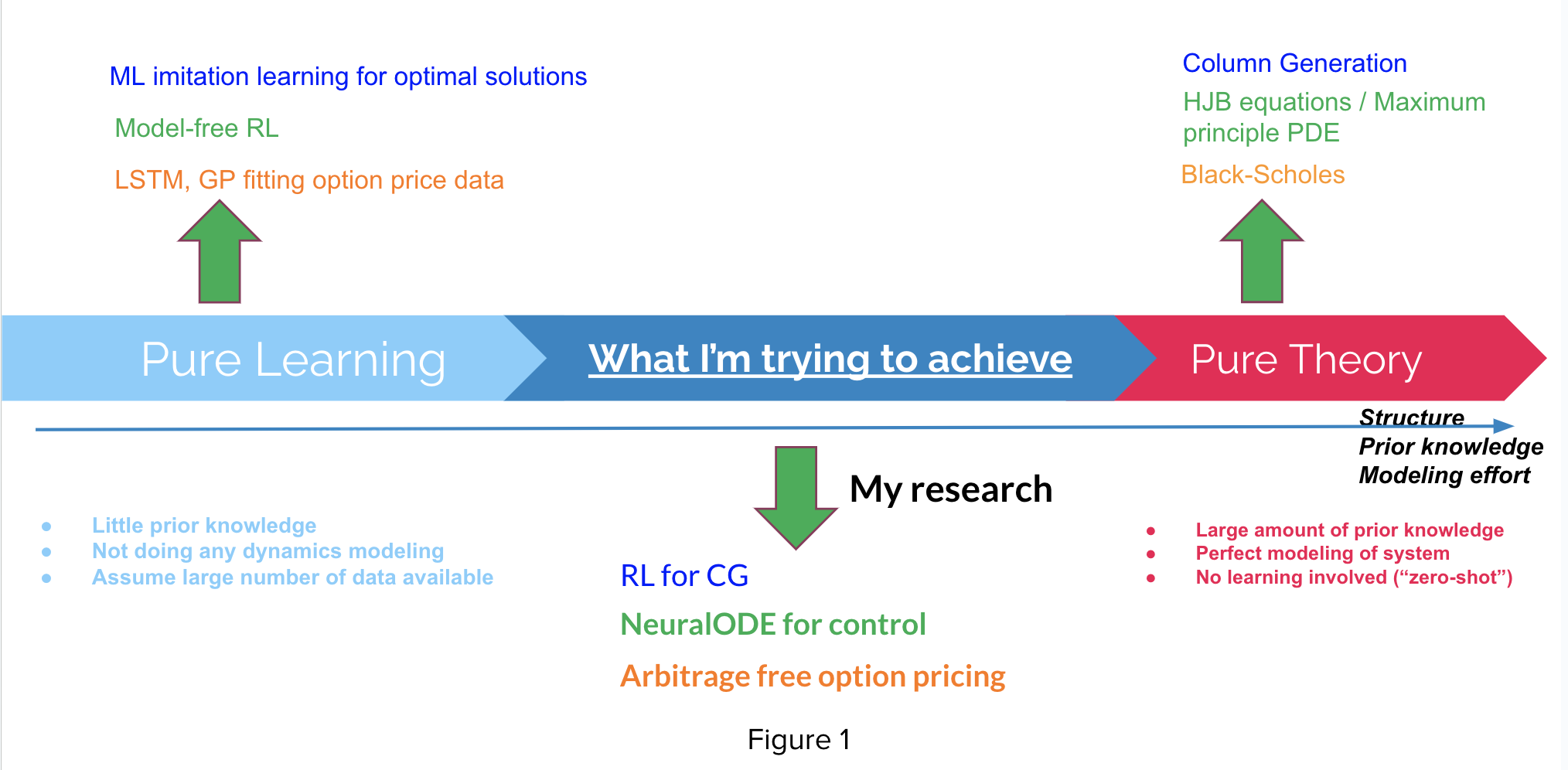
This figure here shows my general research ambition. For any learning task, we can measure the amount of struture or prior knowledge we incorportate in the particular learning method we use, and we put an axis here. On the left-most of this axis, we have “pure learning” methods where we generally learn everything from scratch without any prior modeling about the system, and these methods are easy to set up but require a large amount of training. While on the right-most of this axis we have methods that are “pure theory”, where they generally require a huge effort in defining rigorous mathematical formulation of system dynamics, optimizations or optimality conditions, but once these things are set up, we could analytically solve for optimal solutions without any training.
I want to argue that all the methods on this axis is a particular method that WE CHOOSE to solve the problem (e.g. optimal control / optimization … ) at hand, and the optimal solution method in terms of prior modelling effort is unlikely to lie at the two end-point of this axis but somewhere in the middle for a variety of problems. If we can “theorize” “pure learning” methods or “learningrize” “pure theory” methods, we could potentially hit the optimal trade-off between rigorousness and flexibility, thus achieving optimal solutions or policies with relatively small amount of modelling effort as well as relatively small amount of training effort.
This is what I am trying to pursue in my master study and my research.
Below I will discuss my projects that are directly related to this topic.
RL for CG
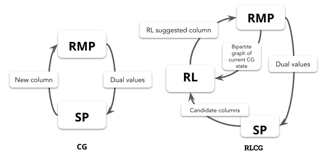
For solving large scale optimization problem (color-coded by dark blue in figure above), “pure learning” method corresponds to train a large neural net directly to output optimal solution from solved optimizations, and a “pure theory” method correpsonds to traditional fixed-rule operational research algorithm column geneartion (CG). By trying to achieve an optimal trade-off between learning and theory, I embed a Reinfocement learning agent inside CG algorithm where agent learn to select varaible to enter the basis optimally, which led to my first project RLCG and my first publication in NeurIPS 2022. The sturcure / prior knowledge I use to achieve such trade-off is the fact that the solution process / optimal basis dynamics is given by CG algorithm rather than a pure generative process or an arbitrary mapping in “pure learning” methods.
I embed a RL agent into column generation algorithm as follows:
Thus the MDP components for RL are the following:

And I denote the above algorithms as RLCG, which is a method lies in the middle of the prior-modelling axis for solving large scale optimization problems. The results below are a direct comparison to the traditional operational research “pure theory” algorithm (denoted as greedy), which always select decision variables that have the most negetive reduced cost. RLCG beats the “pure theory” algorithm as it leads to faster convergence to optimal solutions for different optimization problems (only VRPTW shown here):
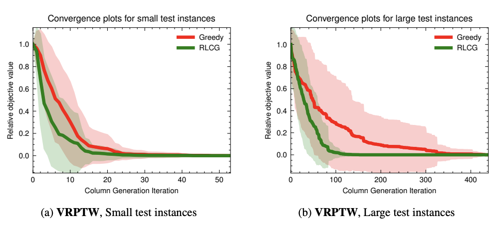
This work is published in NeurIPS 2022.
Machine learning for physical system control
For solving optimal control problem (color-coded by green in figure above), “pure learning” method corresponds to model-free RL where we use countless of interactions with the environment and reward signals to learn a value function or optimize a policy, and a “pure theory” method correpsonds to traditional optimal control method where we model system with controlled differential equations and then derive optimality condition using maximum principle or HJB which are in the form of PDEs, and solving those PDEs will generally lead to optimal controls / policy. By trying to achieve an optimal trade-off between learning and theory, I develop a neural ODE based learning algorithm that can learn the dynamics as well as optimal control at the same time from reletively small amount of interactions from the environment, which led to my thesis work (in preparation) and an application project of irrigation control. The sturcure / prior knowledge I use to achieve such trade-off is the fact that the systems I modelled here are continous in nature and the optimal control is conducted in a vector field.
Neural ODE model
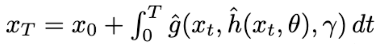
The model that I use is a neural ODE model composed of both a dynamic learner (g) and a controller (h), and how we do a particular trajectory rollout or a prediction is the following:
 The adjoint-method training of dynamic learner and controller is done alternatively so that in the end we are learning both the dynamics of the system as well as the optimal control in that dynamics for some objectives.
Here is an example of a simple control task in a 2-dim state \(x\) and 1-dim control \(u\) environment where the dynamics is given by \(dx/dt = f(x,u) = Ax + Bu\), and we are trying to bring the system from state \((0,0)\) to \((1,-1)\) in shortest time:
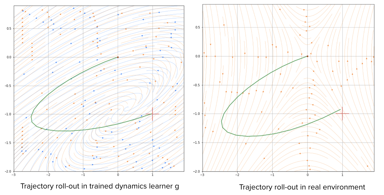
We can see that we successfully bring state to (1,-1), and the vector field or the model we learned by h (shown in oranage arrows) is almost the same as the true dynamics or vector field (shown in blue). The learned controller h is almost the same as analytical optimal control from solving Maximum Principle, but we achieve this without having any knowledge of the true dynamics f(x,u).
Application: Irrigation control
By applying this new continous control method denote as NODEC to the irrigation control problem where dynamics of soil mositure level is given by a particular SDE, I was able to complete a project in India funded by IC-IMPARCS, where I could achieve similar soil moisture evolution and crop yield while saving more than 30% of total water usage compared to an optimization-based method (a “pure theory” method) and farmer’s original irrigations:
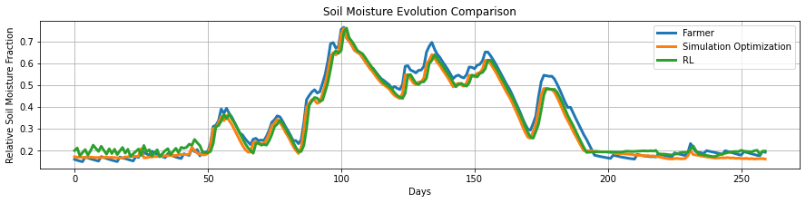
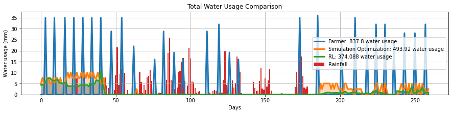
This method (NODEC) is a majority part of my master thesis and the application irrigation project report is in submission to Journal AGU: Advancing earth and space science.
Machine learning for no-arbitrage pricing
For modelling option price (color-coded by orange in figure above), “pure learning” method corresponds to fit a predictive model (either deterministic: LSTM or probabilistic: Gaussian process) using historical data, and a “pure theory” method corresponds to deriving no-arbitrage pricing following the dynamic-hedging arugments with an assumption of underlying asset price process model. By trying to achieve an optimal trade-off between learning and theory, I develop a ML pricing model that parameterize the arbitrage portfolio weights in some particular way so that the training leads to this model learning no-arbitrage prices even if the underlying asset price process is unknown, which led to my current collaboration with NYU Tandon department. The sturcure / prior knowledge I use to achieve such trade-off is the fact that the derivative prices generally, to a good approximation, respect no-arbitrage.
The pricing function learned by no-arbitrage ANN and the delta implied by the same function are the following:
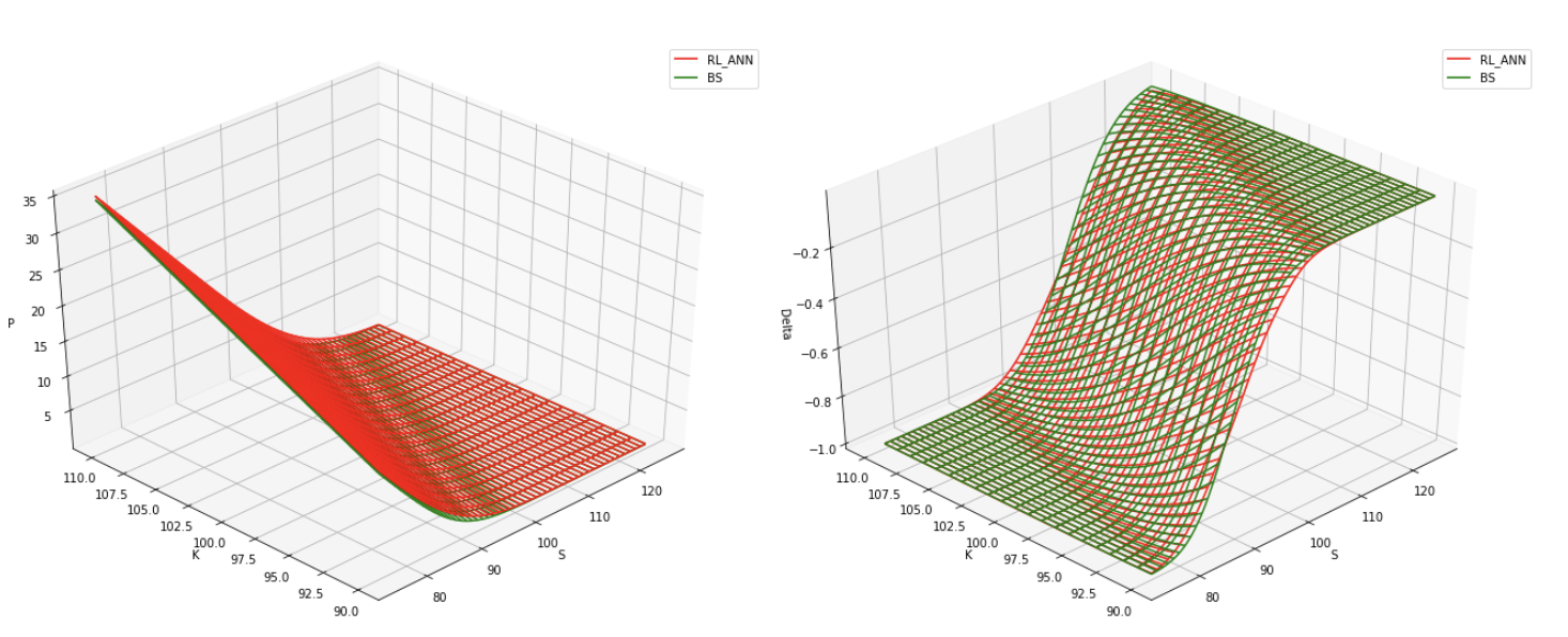 where we recover the analytical no-arbitrage solution without having any knowledge about the true underlying asset process.
By combining this no-arbitrage training with a probabilistic predictive model, we are able to account for fluctuations away from no-arbitrage price in the real-world:
 where we assume that the real option prices distribution has no-arbitrage price mean and Gaussian distributed noise around that mean.
This work is a colloborative work with NYU Tandon department and it is in preparation for submission to Journal of Finance.
Recursive time series data augmentation
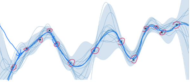
Time series with an unique history can be thought of as one realization of a generally unknown dynamical system. When we try to model such system or when we have some downstream tasks (e.g. time series forecast), what if we don’t have enough prior knowledge about the system to write down equation that governs dynamics of this system, and we also don’t have enough data (we just have one realization) to train a good ML model? How can we now find optimal trade-off between “pure theory”, which is completely unknown here, and “pure learning”, which is prone to overfit here due to lack of data?
In this work, we assume dynamics can be represented by some unknown differential equations, which gives us linearity of the solution. That is, if we take one realization of such dynamics, and take another realization, then the linear combination of these two is again a valid solution or realization of the same dynamical system, and this property holds for all time intervals. We can get different realizations by controlling the weights of linear combination. These intuitions lead us to design a recursive interpolation based time series augmentation method that can augment extreme limited time serues dataset:
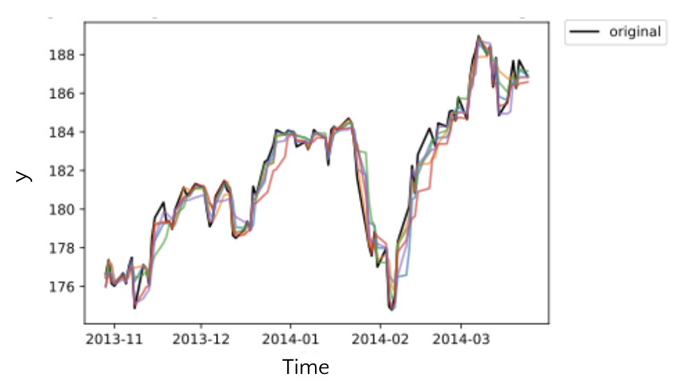 We also prove that the augmented time series (the linear combinations) are bounded within some close distance to the original time series.
However, for many cases, we would like to use the data augmentation to improve downstream learning tasks. For this, we also investigate the relation between learning performance, properties of the time series, and the neural network structure if we use our augmentation on the time series and use all these data to train this nerual network in downstream task.
We also prove that the augmented time series (the linear combinations) are bounded within some close distance to the original time series.
However, for many cases, we would like to use the data augmentation to improve downstream learning tasks. For this, we also investigate the relation between learning performance, properties of the time series, and the neural network structure if we use our augmentation on the time series and use all these data to train this nerual network in downstream task.
The results of downstream task performance improvement is shown here:
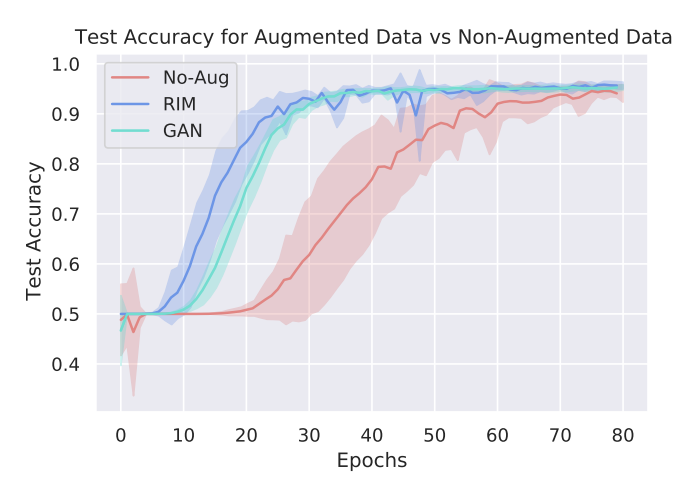 where we show faster convergence and higher accuracy for downstream time series classification task, and we also study time series forecast and Reinforcement learning tasks in our work.
This work is published in ICLR 2023.
Quantum neural ODE for option pricing surface evolution
Simply put: I want to analog-compute option surface evolution with a real quantum state in the physical world, just for fun.
More specifically, this project learns a continuous quantum-circuit evolution whose measurements reproduce an option price surface across maturity.
One-line idea and ideal-world view
Classical option pricing evolves a surface \(V(S,\tau)\) over time-to-maturity \(\tau\). This project instead learns a quantum evolution
$$ |\psi_0\rangle \xrightarrow{U(\theta(\tau))} |\psi_\tau\rangle $$
so that measured basis-state probabilities match the discretized price surface:
$$ V_i(\tau) \propto |\langle i \mid \psi_\tau \rangle|^2 $$
The circuit parameters are not learned independently at each maturity. They are generated by a Neural ODE:
$$ \frac{d\theta}{d\tau} = f_\phi(\theta, \tau) $$
That gives a single continuous trajectory \(\theta(\tau)\), which can be evaluated at any maturity.
What the Neural ODE adds specifically is continuity. Without it, we would just learn one circuit for \(\tau = 0.1\), another for \(\tau = 0.5\), and another for \(\tau = 1.0\). With the Neural ODE, we instead learn a law of motion \(\tau \mapsto \theta(\tau)\).
That means the model is asserting that there is one underlying dynamical mechanism generating the whole family of pricing surfaces across maturity. In that sense, the Neural ODE is doing more than interpolation: it is the object that makes the identification of these different notions of time feel principled.
In the ideal picture, these are all the same time variable:
$$ \text{option surface evolution time} = \text{Neural ODE time} = \text{circuit parameter annealing time} = \text{quantum state evolution time} = \tau $$
So the interpretation is:
market maturity tau
  = Neural ODE evolution parameter
  = quantum circuit control / annealing parameter
  = physical quantum state evolution time
This is the conceptual dream of the project: the option surface does not just get approximated by a quantum model, it evolves along the same idealized time parameter as a real quantum state, if we are controlling the circuit perfectly, for example through a magnetic field strength schedule learned by the Neural ODE under that same time variable.
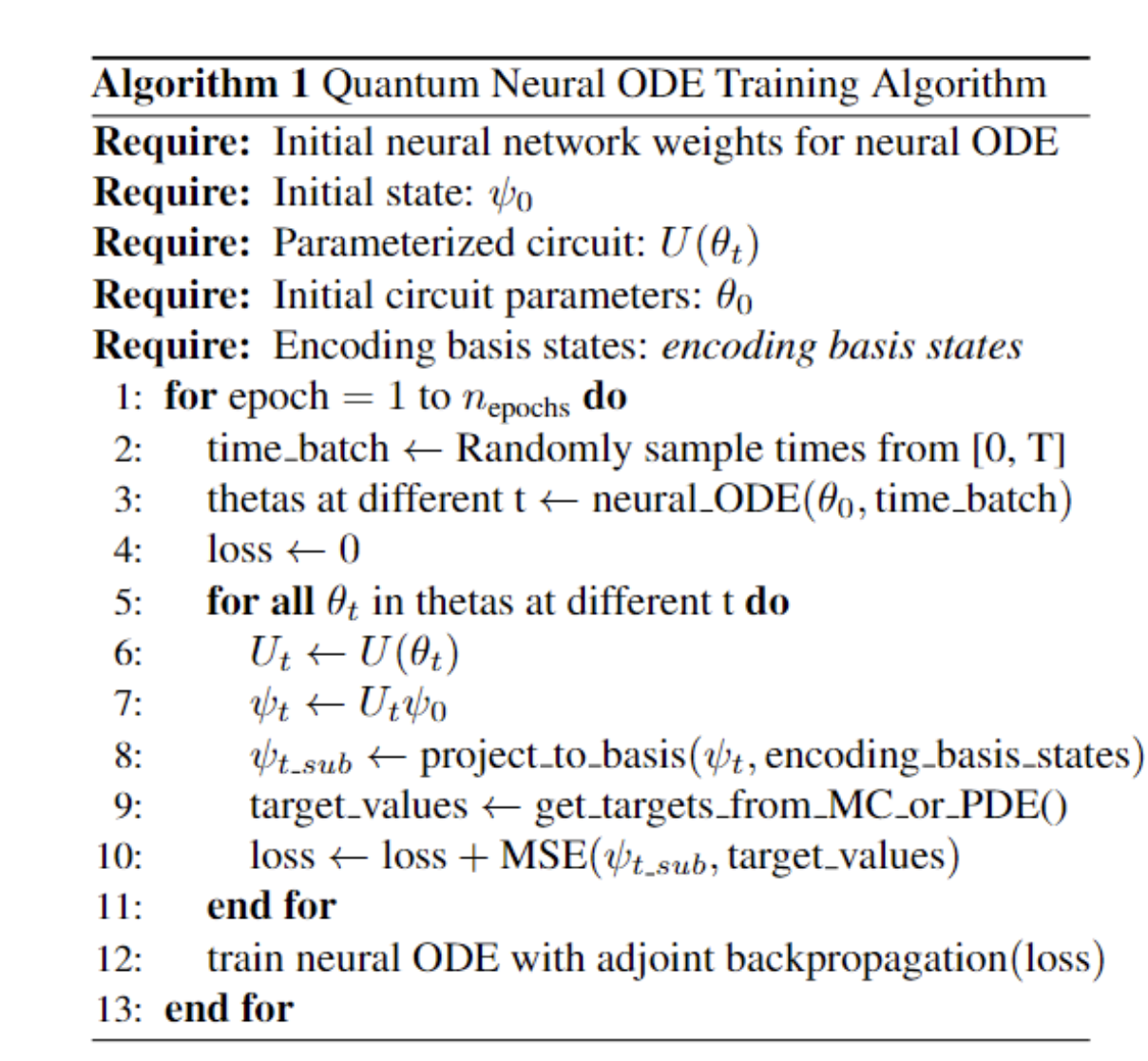
The training setup is illustrated below:
Results and parameter dynamics
We test this method on two pricing models: Black-Scholes with constant volatility (\(\sigma = 0.2\)) and a Local Volatility model where volatility varies linearly from 0.2 to 0.48. The results of fitting the pricing surface evolution in Qiskit simulation are shown below:
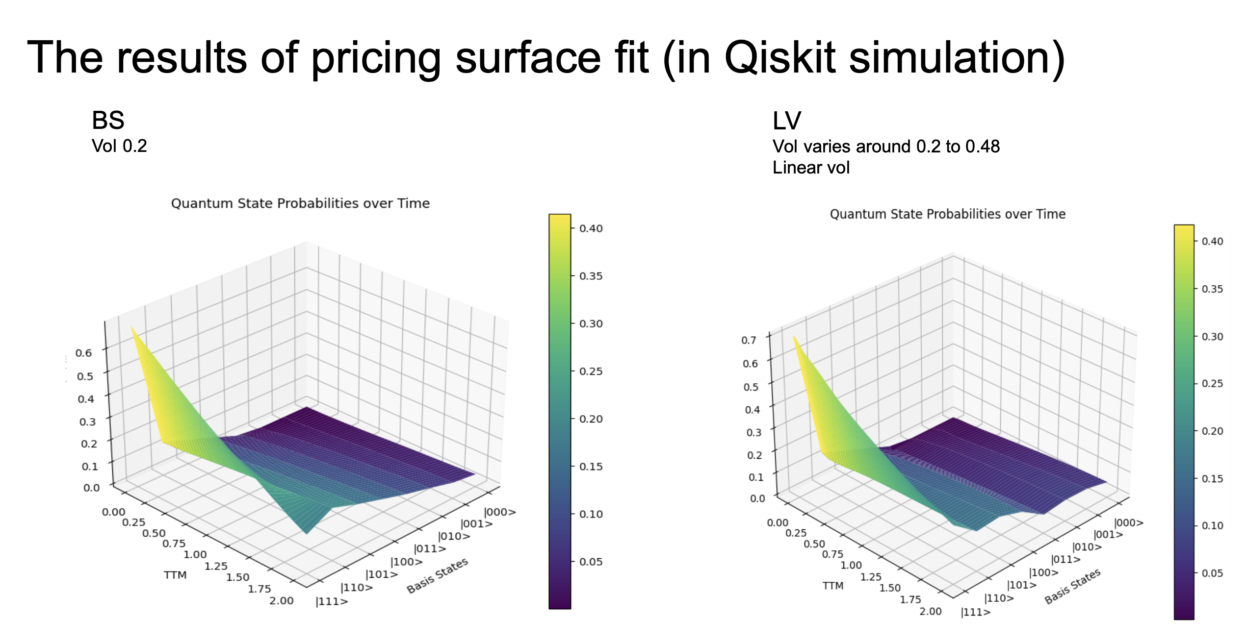
The 3D surfaces show quantum state probabilities (encoding the option prices) over time (TTM axis) and basis states (encoding different strike/moneyness levels). The quantum circuit successfully learns to evolve the initial state so that the resulting probability distribution matches the target pricing surface across all time points, for both the constant-vol BS model and the more complex Local Volatility model.
A key advantage of this approach is that the learned circuit parameter dynamics \(d\theta/dt = f_*(\theta(t))\) reveal interpretable structure about the underlying pricing model. The figure below shows the evolution of quantum circuit parameters over time for both BS and LV models:
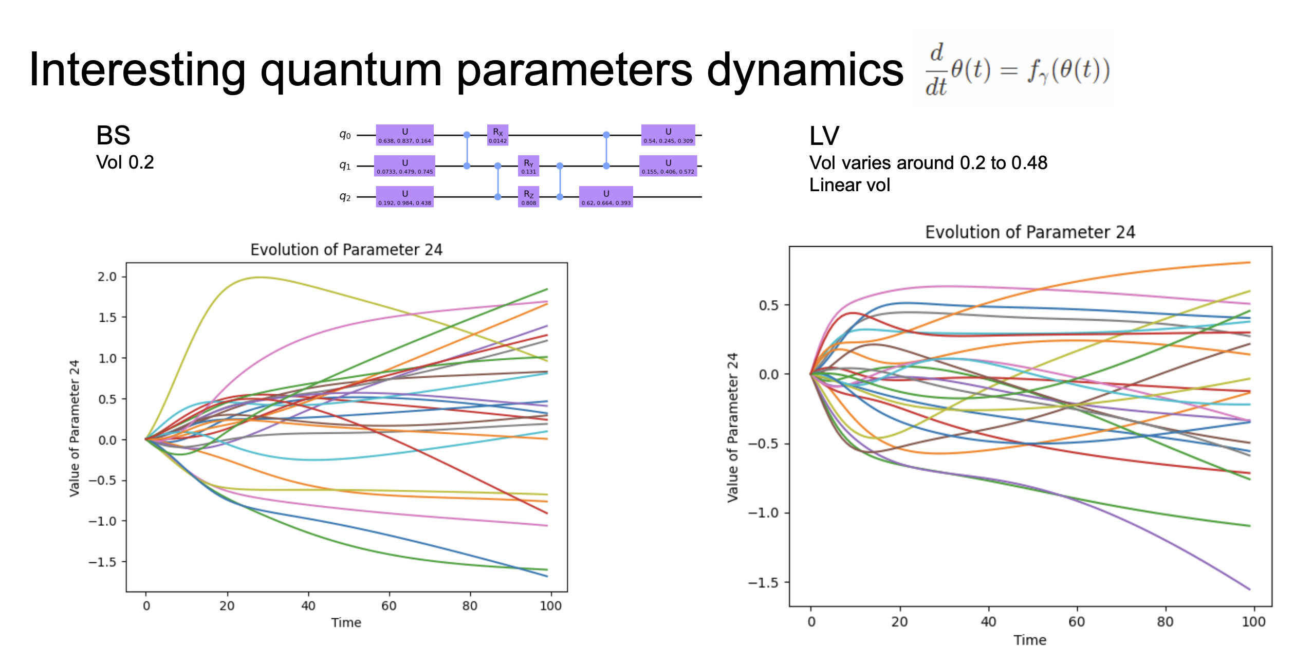
For the BS model (constant vol), the parameter trajectories are smooth and diverge gradually — reflecting the simple, stationary dynamics of the underlying process. For the LV model (time-varying vol), the parameter trajectories exhibit more complex, non-monotonic behavior, reflecting the richer dynamics of a volatility surface that changes with time. The neural ODE autonomously discovers these different dynamical regimes without being told which pricing model generated the data.
We can further examine the angle-encoded dynamics of individual circuit parameters:
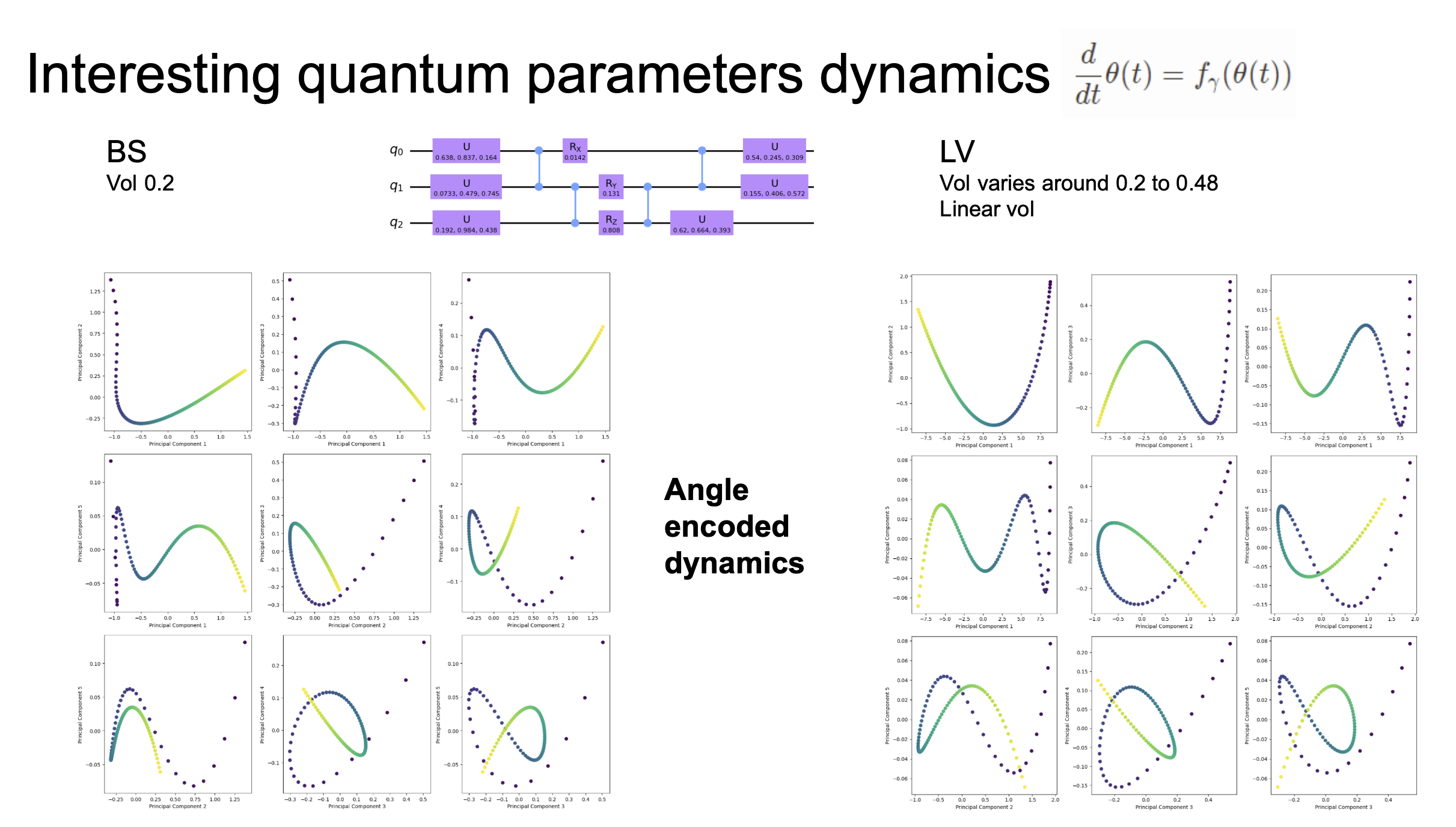
The angle-encoded representations show how individual rotation gate parameters in the quantum circuit evolve over time. The BS model produces smooth, periodic trajectories, while the LV model produces more irregular patterns — the neural ODE adapts the circuit parameter evolution to capture the distinct dynamical signatures of each pricing model.
This achieves the trade-off: we incorporate the structural prior that pricing surfaces evolve continuously under PDE dynamics (via the quantum state evolution under parameterized unitaries), but we do not need to assume any specific stochastic process — the neural ODE learns the correct circuit parameter trajectory from target prices. The quantum circuit provides a physically motivated computational substrate for the evolution, while the neural ODE provides the flexibility to adapt to different pricing dynamics, from simple Black-Scholes to complex Local Volatility models.
The deeper point is that this four-way identification of time is asking whether there exists a time-dependent Hamiltonian \(H(\tau)\) whose quantum evolution reproduces the option-surface dynamics in the measurement basis. If such a mapping exists, then the learned circuit trajectory \(U(\theta(\tau))\) is a discrete, trainable approximation to that generator.
In that sense, the Neural ODE is the bridge that empirically discovers a correspondence between financial diffusion dynamics and quantum unitary dynamics. The learned \(\theta(\tau)\) trajectory becomes the translation layer between the two.
This work was done during my internship at Bloomberg.
Inductive-bias-aware deep tabular learning
For learning on tabular data, “pure learning” method corresponds to using a generic deep neural network (e.g. MLP) that treats the input as a flat vector and learns all feature interactions from scratch, and a “pure theory” method corresponds to hand-crafted feature engineering combined with simple models (linear or tree-based) that make strong structural assumptions about the data. By trying to achieve an optimal trade-off between learning and theory, I develop a non-linear LassoNet architecture that respects the known inductive biases of tabular data while retaining the representational power of deep learning. The structure / prior knowledge I use to achieve such trade-off is the set of inductive biases specific to tabular data.
Tabular data has well-known inductive biases that differ fundamentally from images or text:
- Feature heterogeneity: each feature has its own semantic meaning, scale, and distribution — unlike pixels or tokens which share a common representation space.
- Feature sparsity: not all features are relevant, and the model should be able to select or suppress features rather than being forced to use all of them.
- Irregular feature interactions: interactions between features are not spatially local (as in images) or sequential (as in text), but can be arbitrary and sparse.
Standard deep learning architectures ignore these biases. MLPs treat features as interchangeable dimensions in a flat vector. Transformers applied naively to tabular data create attention over features but do not enforce sparsity or heterogeneity. Tree-based methods (“pure theory” side) naturally respect these biases through axis-aligned splits and feature selection, which is why they remain dominant on many tabular benchmarks.
NonlinearLasso architecture
Our architecture, NonlinearLasso, respects all three inductive biases through a three-module design:
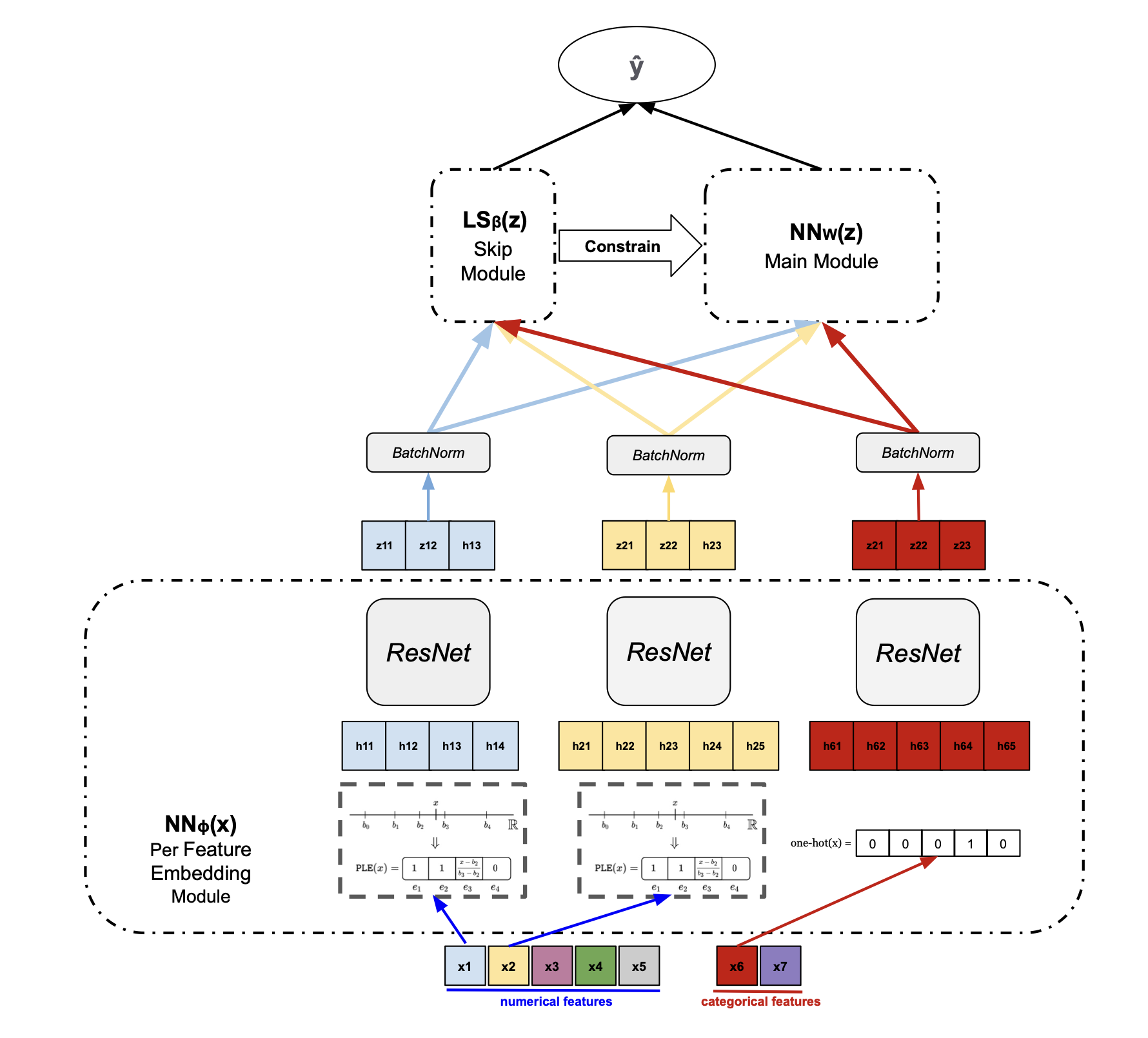
The architecture consists of three modules stacked bottom-to-top:
- Per-Feature Embedding Module \(\text{NN}_\theta(x)\) (bottom): each feature is independently embedded using its own ResNet block. Numerical features are first discretized into bins and categorical features are one-hot encoded, then each feature group passes through a dedicated ResNet followed by BatchNorm. This respects feature heterogeneity — each feature gets its own learned non-linear representation with its own parameters, analogous to how each feature in a tree model is treated independently at each split. The per-feature ResNet embeddings produce representations \(z = \{z_1, \ldots, z_p\}\) that are passed to the upper modules.
- Main Module \(\text{NN}_w(z)\) (top right): the embedded features are passed through a deep network that learns non-linear cross-feature interactions. This is the “learning” component that gives the model representational power beyond what tree-based methods can achieve.
- Skip Module \(\text{LS}_\beta(z)\) (top left): a linear skip connection from the embedded features directly to the output, with coefficients \(\beta_j\) for each feature. Crucially, there is a hierarchy constraint between the skip and main modules: the main module’s use of feature \(j\) is constrained by the skip module’s coefficient for that feature. Formally, \(\|W_j^{(1)}\|_\infty \leq M |\beta_j|\), where \(W_j^{(1)}\) is the main module’s first-layer weight for feature \(j\), \(\beta_j\) is the skip connection coefficient, and \(M\) is a hierarchy parameter. If \(\beta_j = 0\), the feature is entirely removed from both the linear and non-linear paths — enforcing feature sparsity in a principled way.
The final prediction is: \(\hat{y} = \text{LS}_\beta(z) + \text{NN}_w(z)\), combining the linear skip path with the deep non-linear path under the hierarchy constraint.
The key difference from the original LassoNet is that our model is non-linear in its treatment of feature embeddings and interactions. The per-feature ResNet embeddings and the deep main module allow the model to learn complex, non-linear feature transformations and cross-feature interactions, while the LassoNet-style hierarchy constraint ensures that the model still performs global feature selection and maintains interpretability.
Benchmarking results
We benchmark NonlinearLasso against a comprehensive set of tree-based models (CatBoost, XGBoost, LightGBM, RandomForest, DecisionTree), deep tabular models (NODE, DANet, SAINT, TabNet, TabTransformer, FTTransformer, rtdl_ResNet, rtdl_MLP, STG, VIME, DeepFM), and classical methods (KNN, SVM, LinearModel) across multiple tabular datasets:
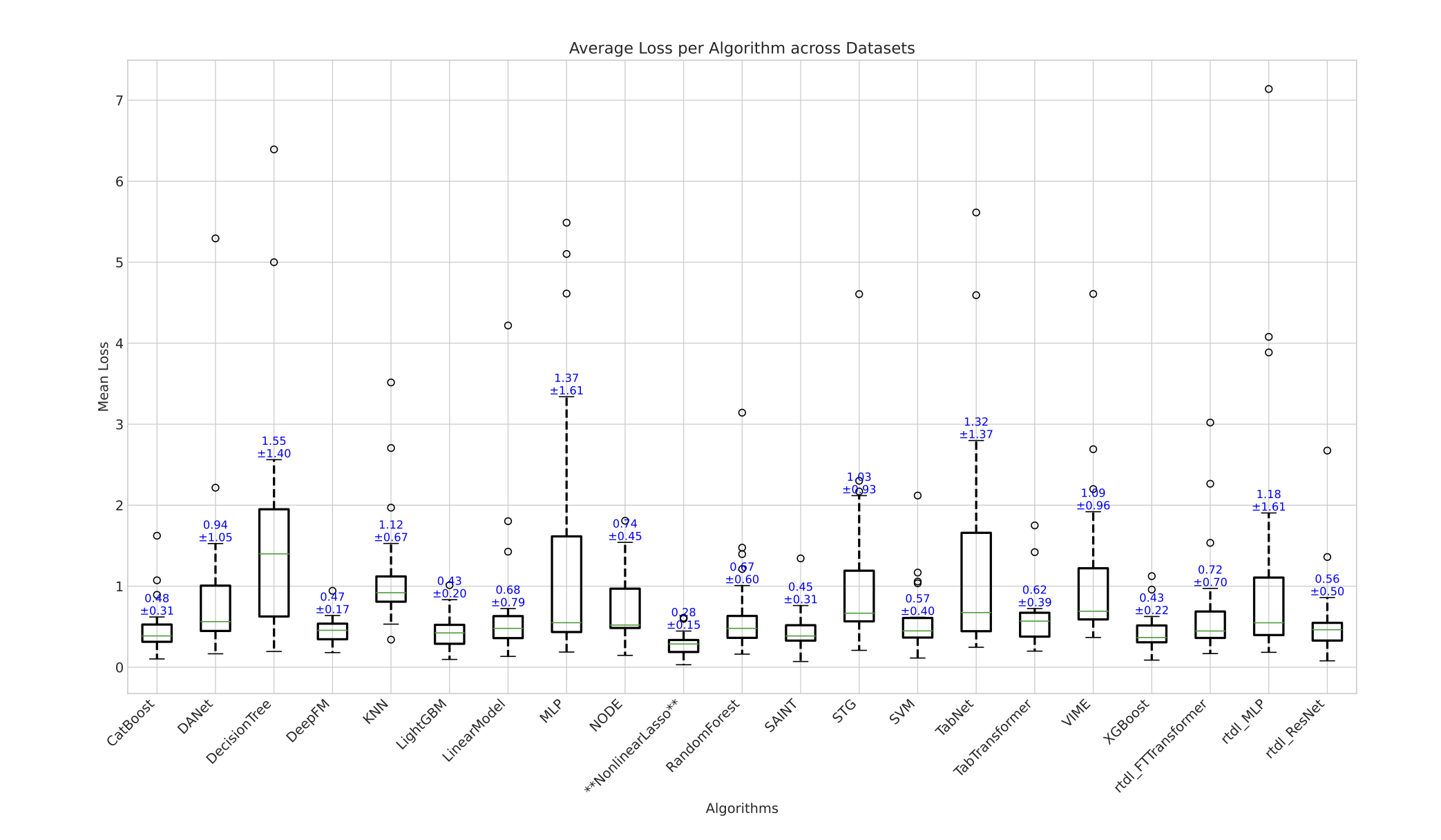
NonlinearLasso achieves the lowest average loss (\(0.28 \pm 0.15\)) across all datasets, substantially outperforming both tree-based champions like LightGBM (\(0.43 \pm 0.20\)) and XGBoost (\(0.93 \pm 0.22\)), as well as all deep tabular competitors including SAINT (\(0.45 \pm 0.31\)), TabTransformer (\(0.62 \pm 0.39\)), FTTransformer (\(0.72 \pm 0.22\)), and NODE (\(0.94 \pm 0.45\)). Notably, NonlinearLasso also has the tightest variance, indicating consistent performance across diverse tabular datasets rather than excelling on some and failing on others.
This architecture achieves the optimal trade-off: we incorporate the structural priors that tree-based models use (feature independence via per-feature embedding, sparsity via hierarchy-constrained feature selection, heterogeneous treatment of features via dedicated ResNets) into a deep learning architecture, without sacrificing the representational power that comes from learned non-linear embeddings and deep cross-feature interactions. The result is a model that consistently outperforms both sides of the prior-modelling axis.
This work was done during my internship at Borealis AI (RBC). To paper
Systemic risk mitigation in financial networks
Quantum annealing for optimization of network structure
In highly connected fnancial networks, the failure of a single or a few institution can cascade into additional
bank failures:
 This systemic risk can be mitigated by adjusting the loans, holding shares, and other
liabilities connecting institutions in a way that prevents cascading of failures. We are approaching the
systemic risk problem by attempting to optimize the connections between the institutions with financially meaningful objective and constraints:
This systemic risk can be mitigated by adjusting the loans, holding shares, and other
liabilities connecting institutions in a way that prevents cascading of failures. We are approaching the
systemic risk problem by attempting to optimize the connections between the institutions with financially meaningful objective and constraints:
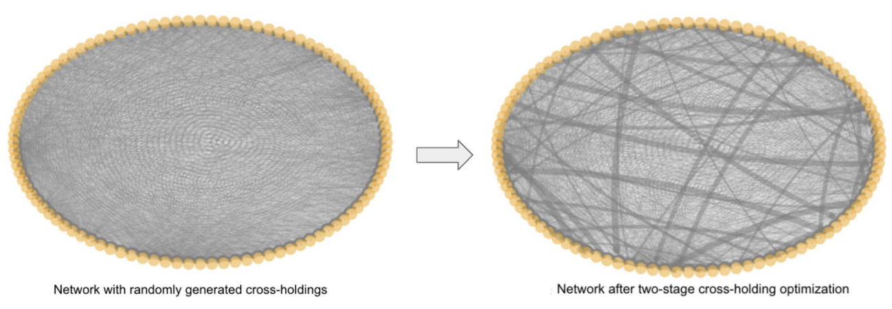 We notice that the cascade failures first spread through highly connected groups (a module) and then spread between modules, as the connection between banks are the brigde that failure spreads. This intution leads us to the two-stage cascade prevention method, where we would first partition financial networks into modulues (community detection), and then optimize the module sub-network connections individually. In this way, we could
confine cascade failures from its source and keep the change of connections to a minimum.
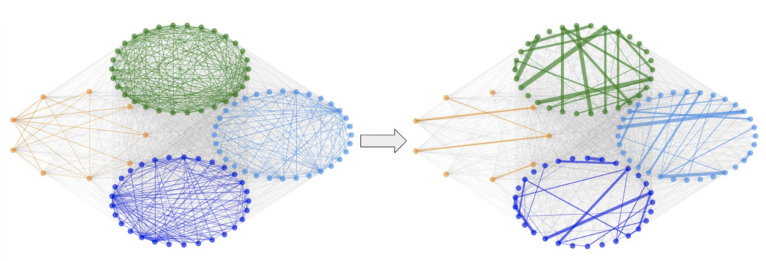 We apply quantum annealing as our heuristic for community detection where it can achieve more accurate partitioning with less time complexity. In particular, the modularity maximization is formullated as QUBO, mapped to Pegasus embedding and then solved in D-wave Advantage Quantum Annealer.
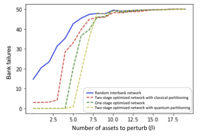
The cascade simulation is mitigated as a result of our method, indicated by delayed phase transition in cascade failures where financial network can withstand higher perturbation without failure:
We apply quantum annealing as our heuristic for community detection where it can achieve more accurate partitioning with less time complexity. In particular, the modularity maximization is formullated as QUBO, mapped to Pegasus embedding and then solved in D-wave Advantage Quantum Annealer.
The cascade simulation is mitigated as a result of our method, indicated by delayed phase transition in cascade failures where financial network can withstand higher perturbation without failure:
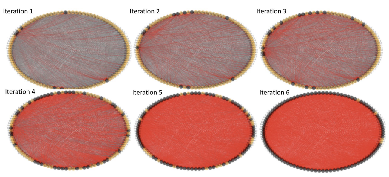
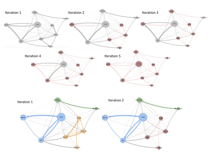
 We also demonstrate similar results using real-world data, where we perturb the original network and optimized network with the same level of perturbation, and compare the cascade results. We can see that all the institutions in the original network (top) fail as a result of the perturbation while in the optimized network (bottom) only few institutions fail.
This work is published in Nature Scientific Report on March, 2023.
Central bank cascade free control
This work is a direct extension from previous work on cascade failure mitigation. Instead of posing change in connectivities between institutions (banks in this case) as a hard constraints on banks, we respect the objective of banks which is maximizing their own profits. Therefore, central bank aims to give incentives or penalties as control signal to the system whose dynamics are given by the zero-sum games formulated as individual banks’ greedy optimizations.
We already studied some property of such dynamical system we are trying to control, where for some particular controls we have converged Nash Equilibrium of the low level optimizations (banks), while for some other controls we have oscillation between equilibria:
 We are now in the stage of learning an optimal control corresponds to cascade-free trajectory of this compicated dynamical system.